PandasとStatsModelsを使って飛行機乗客数の時系列分析を行う
時系列分析(Python)
jupyter notebookを利用し、以下の手順で記載しています。
- ライブラリーのインポートとグラフ描画準備 ...[1,2]
- Pandasで分析用データの読み込み(CSVファイルを利用) ...[3,4]
- 乗客数の時系列データをグラフで確認 ...[5]
- トレンド、季節、残差成分に分離してデータを可視化 ...[6]
- 対数変換したデータもグラフで確認 ...[7]
- 自己相関(acf)と偏自己相関(pacf)をグラフで確認 ...[8]
- SARIMAモデルの作成(季節自己回帰和分移動平均) ...[9]
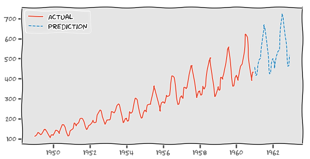
- モデルを使って未来データを予測、グラフ化 ...[10-12]
In [1]:
# ライブラリーインポート、グラフ描画準備
import numpy as np
import pandas as pd
import matplotlib.pyplot as plt
import statsmodels.api as sm
% matplotlib inline
plt.style.use('ggplot')
plt.xkcd()
Out[1]:
In [2]:
# statsmodelsのバージョン確認
sm.version.full_version # SARIMAX利用に0.8.0以上が必要
Out[2]:
In [3]:
# PandasでCSVファイルを読み込む
# 『AirPassengers.csv』は以下の外部サイトよりダウンロードしたファイルを利用
# https://www.analyticsvidhya.com/wp-content/uploads/2016/02/AirPassengers.csv

df = pd.read_csv('AirPassengers.csv',
                 index_col=0, parse_dates=[0], dtype='float')

print(len(df)) # 144データ(1949年1月から1960年12月まで、月毎の飛行機乗客数)
df.head()
Out[3]:
In [4]:
# pandasのSeriesに乗客数データを格納
ts = df['#Passengers']
In [5]:
# 乗客数データをグラフで可視化(pandas.plot)
ts.plot(figsize=(8, 2))
Out[5]:

In [6]:
# オリジナル ->トレンド成分、季節成分、残差成分に分解してプロット
res = sm.tsa.seasonal_decompose(ts)

trend = res.trend
seasonal = res.seasonal
residual = res.resid

plt.figure(figsize=(8, 8))

# オリジナルの時系列データプロット
plt.subplot(411)
plt.plot(ts)
plt.ylabel('Original')

# trend のプロット
plt.subplot(412)
plt.plot(trend)
plt.ylabel('Trend')

# seasonal のプロット
plt.subplot(413)
plt.plot(seasonal)
plt.ylabel('Seasonality')

# residual のプロット
plt.subplot(414)
plt.plot(residual)
plt.ylabel('Residuals')

plt.tight_layout()

In [7]:
# log変換データで確認
ts_log = np.log(ts)
res_log = sm.tsa.seasonal_decompose(ts_log)
trend_log = res_log.trend
seasonal_log = res_log.seasonal
residual_log = res_log.resid
plt.figure(figsize=(8, 8))
# オリジナルlog変換
plt.subplot(411)
plt.plot(ts_log, c='b')
plt.ylabel('Original')
# trend
plt.subplot(412)
plt.plot(trend_log, c='b')
plt.ylabel('Trend')
# seasonal
plt.subplot(413)
plt.plot(seasonal_log, c='b')
plt.ylabel('Seasonality')
# residual
plt.subplot(414)
plt.plot(residual_log, c='b')
plt.ylabel('Residuals')
plt.tight_layout()

In [8]:
# 自己相関(acf)のグラフ
fig = plt.figure(figsize=(8, 8))
ax1 = fig.add_subplot(211)
fig = sm.graphics.tsa.plot_acf(ts, lags=48, ax=ax1)
# 偏自己相関(pacf)のグラフ
ax2 = fig.add_subplot(212)
fig = sm.graphics.tsa.plot_pacf(ts, lags=48, ax=ax2)
plt.tight_layout()

In [9]:
# SARIMAモデル(季節自己回帰和分移動平均モデル)
#import warnings
#warnings.filterwarnings('ignore') # warnings非表示
srimax = sm.tsa.SARIMAX(ts, order=(2,1,3),
                            seasonal_order=(0,2,2,12),
                            enforce_stationarity = False,
                            enforce_invertibility = False
                           ).fit()
# order=(2,1,3), season=(0,2,2)  -> aic 705.953
# print(srimax.summary())
# Warnings:
# [1] Covariance matrix calculated using the outer product of gradients (complex-step).
In [10]:
# 未来データ予測
pred = srimax.forecast(24) # 未来の24データ予測
pred[:10]
Out[10]:
In [11]:
# 未来データ予測
pred = srimax.forecast(24) # 未来の24データ予測

# 実データと予測データのグラフ描画
plt.figure(figsize=(10, 5))
plt.plot(ts, label='Actual')
plt.plot(pred, label='Prediction', linestyle='--')
plt.legend(loc='best')
Out[11]:
In [12]:
# データ予測(期間指定)
predict_fromTo = srimax.predict('1954-01-01', '1962-12-01')

# 実データと予測データのグラフ描画
plt.figure(figsize=(10, 5))
plt.plot(ts, label='Actual')
plt.plot(predict_fromTo, label='Prediction', alpha=0.5)
plt.legend(loc='best')
Out[12]:

詳細は以下の記事にも記載しています。
〜 モモノキ&ナノネと学習シリーズ(時系列分析) 〜
スポンサーリンク


0 件のコメント :
コメントを投稿